The Three Stages of Concrete Behavior Under loading: The Fundamentals of Concrete Design

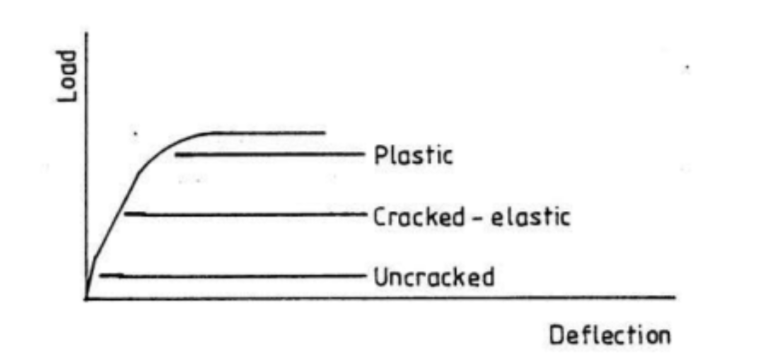
Concrete design in civil engineering is guided by standards like Eurocode 2 and ACI, which help engineers determine the appropriate reinforcement to ensure structural integrity and safety. The underlying principle of concrete design is based on the behavior of concrete under-loading. Reinforced Concrete, the main load-bearing concrete construction material, exhibits three key stages of behavior when loaded from initial loading stages to failure. This post will explore the three key stages of concrete behavior in reinforced concrete sections: Stage I (Uncracked), Stage II (Cracked Serviceability State), and Stage III (Ultimate Limit State).

Key Definitions and Symbols

– $f_{ck}$ : Characteristic compressive strength of concrete

– $f_{yk}$ : Characteristic yield strength of reinforcement steel

– $\sigma_s$ : Stress in the reinforcement steel

– $\sigma_c$ : Stress in the concrete

– $x$ : Depth of the neutral axis

– $d$ : Effective depth of the section

– $A_s$ : Area of tensile reinforcement

– $A_s'$ : Area of compression reinforcement

– $M$ : Bending moment

– $k$ : Ratio of the neutral axis depth to the effective depth

– h = overall depth of the section

-d = effective depth, i.e. depth from the compression face to the centroid of tension steel

-b = breadth of the section

-x = depth to the neutral axis

-fs = stress in steel

-fc = stress in concrete

-As = area of tension reinforcement

-εcu3 = maximum strain in the concrete

-εs = strain in steel

The example focuses on balanced and singly reinforced states for concrete beams.

Stage I: Uncracked (Elastic Behavior)

In this initial stage, the concrete section is considered uncracked and behaves elastically under low-stress levels. This state is suitable for cases of small loads and where the cracks are prevented from occurring.

Key Assumptions

– Concrete and steel both respond linearly/elastic under low stresses.

-Bernoulli’s hypothesis is satisfied i.e the strain distribution is linear

-Hooks law is satisfied or the material is elastic: i.e

$\sigma = E \cdot \epsilon$

– The entire cross-section contributes to load resistance.

– The tensile strength of concrete is not exceeded, so no cracks develop.

The Naviers equation is used to calculate the stress of steel

-Converting steel area to an equivalent concrete area using a modular ratio

$\alpha = \frac{E_s}{E_c}$

-The neutral axis is x=(α−1)⋅As+bh(α−1)⋅As⋅d+21bh2

-Neutral Axis $x$ Formula

The depth of the neutral axis $x$ can be expressed as:

$x = \frac{(\alpha - 1) \cdot A_s \cdot d + \frac{1}{2} b h^2}{(\alpha - 1) \cdot A_s + b h}$

where:

– $\alpha = \frac{E_s}{E_c}$ is the modular ratio,

– $A_s$ is the area of the steel reinforcement,

– $b$ is the width of the concrete section,

– $h$ is the height of the concrete section,

– $d$ is the distance from the section’s top to the steel reinforcement’s centroid.

Moment of Inertia $I$ Formula

The moment of inertia $I$ about the neutral axis is:

$I = \frac{b \cdot h^3}{12} + b \cdot h \left( x - \frac{h}{2} \right)^2 + (\alpha - 1) \cdot A_s \cdot (d - x)^2$

where:

– The first term, $\frac{b \cdot h^3}{12}$ , is the moment of inertia of the concrete section about its centroidal axis,

– The second term, $b \cdot h \left( x - \frac{h}{2} \right)^2$ , shifts the concrete area’s moment of inertia to the neutral axis,

– The third term, $(\alpha - 1) \cdot A_s \cdot (d - x)^2$ , is the moment of inertia of the transformed steel area about the neutral axis

-The stresses in concrete

The concrete stress ( f_c ) in terms of the bending moment ( M ), the moment of inertia ( I ), the distance ( x ) from the neutral axis, and the section width ( b ) is expressed as :

$f_c = \frac{M}{I} \cdot x$

where:

( f_c ): The stress in the concrete,
( M ): The bending moment,
( I ): The moment of inertia of the section about the neutral axis,
( x ): The distance from the neutral axis .

The expression for $\alpha_{cc}$ can be written as:

$f_c = \frac{M}{I_{\text{id}}} \cdot x$

where:

– $M$ represents the bending moment,

– $I_{\text{id}}$ represents a moment of inertia

– $x$ is the distance from the neutral axis.

The stresses in steel

$f_t = \frac{M}{I_{\text{id}}} \cdot (h - x)$

where:

– $M$ is bending moment,

– $I_{\text{id}}$ represents a moment of inertia ,

– $h$ is height of the section,

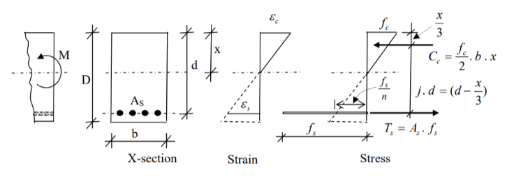
Stage II: Cracked (Serviceability State) also called the work stress method

In Stage II, the concrete’s tensile stress exceeds its tensile strength, leading to cracks in the concrete section. However, the structure remains functional, and serviceability requirements must be satisfied.

Key Assumptions

-Bernoulli’s hypothesis is satisfied i.e the strain distribution is linear

-Hooks law is satisfied or the material is elastic: i.e

$\sigma = E \cdot \epsilon$

– Cracking occurs in the tensile region, but the section retains serviceability.

– Concrete in tension is neglected; only steel reinforcement takes tension.

– Stress distribution in the compression zone is linear.

Design Equations for Singly Reinforced Rectangular Section

In a singly reinforced rectangular section, reinforcement is provided only on the tension side. Here are the key steps and equations for determining the neutral axis depth, stress relationships, and moment of resistance.

Assumptions

1. Concrete in tension is neglected, so the reinforcement carries all the tensile stress.

2. Both concrete and steel behave elastically within the working stress range.

3. A perfect bond exists between steel and concrete.

Variables

– $b$ : Width of the section

– $d$ : Effective depth (distance from the top fiber to the center of the reinforcement)

– $A_s$ : Area of steel reinforcement

– $f_c$ : Compressive stress in concrete

– $f_s$ : Tensile stress in steel

– $x$ : Depth of the neutral axis from the top of the section

– $M$ : Applied bending moment

– $n = \frac{E_s}{E_c}$ : Modular ratio (ratio of Young’s modulus of steel to that of concrete)

a) Determining Neutral Axis Depth $x$

1. Strain Compatibility

From the strain diagram, the ratio of strains in concrete and steel is given by the similarity of triangles:

$\frac{\epsilon_s}{\epsilon_c} = \frac{d - x}{x}$

where $\epsilon_s$ is the strain in steel and $\epsilon_c$ is the strain in concrete.

2. Stress-Strain Relationship (Hooke’s Law)

In the elastic range, applying Hooke’s law:

$\epsilon_c = \frac{f_c}{E_c} \quad \text{and} \quad \epsilon_s = \frac{f_s}{E_s}$

Since the modular ratio $n$ is defined as $n = \frac{E_s}{E_c}$ , we can write:

$\frac{\epsilon_s}{\epsilon_c} = n \cdot \frac{f_c}{f_s} = \frac{d - x}{x}$

3. Neutral Axis Depth $x$

Solving for $x$ in terms of the modular ratio $n$ , concrete stress $f_c$ , and steel stress $f_s$ :

$\frac{x}{d} = \frac{n \cdot f_c}{n \cdot f_c + f_s} = k$

where $k = \frac{x}{d}$ is a ratio indicating the position of the neutral axis. Thus:

$x = k \cdot d$

b) Equilibrium of Internal Forces

To maintain equilibrium, the compressive force in the concrete $C$ must equal the tensile force in the steel $T$ :

1. Compressive Force in Concrete

The compressive force $C$ is given by:

$C = \frac{f_c \cdot b \cdot x}{2}$

2. Tensile Force in Steel

The tensile force $T$ in the steel is:

$T = A_s \cdot f_s$

3. Equilibrium Condition

Setting $C = T$ :

$\frac{f_c \cdot b \cdot x}{2} = A_s \cdot f_s$

Substituting $x = k \cdot d$ :

$\frac{f_c \cdot b \cdot k \cdot d}{2} = A_s \cdot f_s$

4. Steel Ratio $\rho$

Defining the geometric steel ratio $\rho = \frac{A_s}{b \cdot d}$ , we can substitute $A_s = \rho \cdot b \cdot d$ :

$f_s = \frac{2 f_c \cdot k}{\rho}$

c) Moment of Resistance

The moment of resistance $M$ is determined by taking moments of the internal forces about the neutral axis or the center of compression.

1. Lever Arm

The lever arm $j \cdot d$ is the distance between the line of action of the compressive and tensile forces. It can be defined as:

$j = 1 - \frac{k}{3}$

2. Moment of Resistance (Concrete Stress)

The moment of resistance $M$ in terms of the concrete stress $f_c$ is:

$M = \frac{f_c \cdot b \cdot x}{2} \cdot j \cdot d = f_c \cdot b \cdot k \cdot d^2 \cdot \left(1 - \frac{k}{3}\right)$

3. Moment of Resistance (Steel Area)

Alternatively, the moment of resistance in terms of the area of steel $A_s$ and steel stress $f_s$ is:

$M = A_s \cdot f_s \cdot j \cdot d$

Substituting $j = 1 - \frac{k}{3}$ :

$M = A_s \cdot f_s \cdot d \cdot \left(1 - \frac{k}{3}\right)$

Summary of Key Equations

– Neutral Axis Depth $x$ :

$x = \frac{n \cdot f_c \cdot d}{n \cdot f_c + f_s}$

– Force Equilibrium:

$\frac{f_c \cdot b \cdot x}{2} = A_s \cdot f_s$

– Moment of Resistance (Concrete Stress):

$M = f_c \cdot b \cdot k \cdot d^2 \cdot \left(1 - \frac{k}{3}\right)$

– Moment of Resistance (Steel Area):

$M = A_s \cdot f_s \cdot d \cdot \left(1 - \frac{k}{3}\right)$

These equations provide the fundamental relationships for analyzing and designing singly reinforced rectangular sections under bending.

The expression for $k$ :

$k = -(\rho \cdot n) + \sqrt{(\rho \cdot n)^2 + (2 \rho \cdot n)}$

is derived from a quadratic equation that typically arises in analyzing a singly reinforced concrete section.

Derivation of $k$ Using Force Equilibrium

1. Force Equilibrium in the Section:

For a singly reinforced rectangular section, the compressive force in the concrete $C$ must balance the tensile force in the steel $T$ .

2. Expressing Forces:

– The compressive force $C$ in the concrete (assuming a rectangular stress block) is:

$C = 0.5 \cdot f_c \cdot b \cdot x$

where $f_c$ is the concrete stress, $b$ is the width of the section, and $x$ is the depth of the neutral axis.

– The tensile force $T$ in the steel reinforcement is:

$T = A_s \cdot f_s$

where $A_s$ is the area of the steel reinforcement, and $f_s$ is the stress in the steel.

3. Using the Modular Ratio and Reinforcement Ratio:

– Define the modular ratio $n = \frac{E_s}{E_c}$ , where $E_s$ and $E_c$ are the moduli of elasticity for steel and concrete, respectively.

– Let $\rho = \frac{A_s}{b \cdot d}$ , where $A_s$ is the area of the steel reinforcement and $d$ is the effective depth.

4. Setting Up the Equilibrium Equation:

Since $C = T$ , we have:

$0.5 \cdot f_c \cdot b \cdot x = A_s \cdot f_s$

5. Expressing $f_s$ in terms of $f_c$ :

Using the relationship $f_s = n \cdot f_c$ , we get:

$0.5 \cdot f_c \cdot b \cdot x = \rho \cdot b \cdot d \cdot (n \cdot f_c)$

6. Solving for $k = \frac{x}{d}$ :

Cancelling $f_c$ and $b$ , we obtain:

$0.5 \cdot x = \rho \cdot n \cdot d$

By substituting $x = k \cdot d$ , this equation can be rearranged into a standard quadratic form:

$k^2 - (\rho \cdot n) \cdot k - (2 \rho \cdot n) = 0$

7. Solving the Quadratic Equation:

Solving for $k$ using the quadratic formula $k = \frac{-b \pm \sqrt{b^2 - 4ac}}{2a}$ , with $a = 1$ , $b = -\rho \cdot n$ , and $c = -2 \rho \cdot n$ , gives:

$k = -(-\rho \cdot n) \pm \sqrt{(\rho \cdot n)^2 + 2 \rho \cdot n}$

Simplifying this, we get:

$k = (\rho \cdot n) + \sqrt{(\rho \cdot n)^2 + 2 \rho \cdot n}$

Since we are looking for the positive root that gives a physical result, we discard the negative option:

$k = -(\rho \cdot n) + \sqrt{(\rho \cdot n)^2 + 2 \rho \cdot n}$

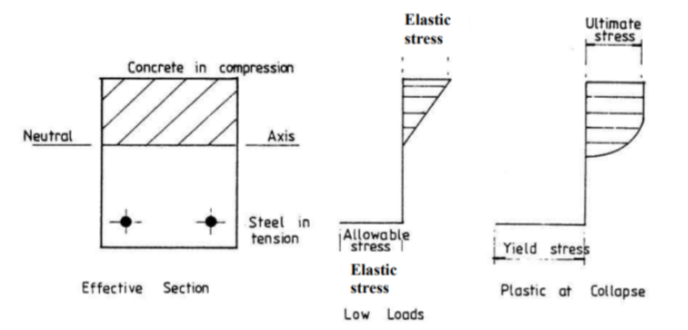
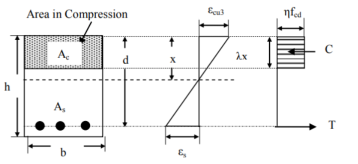
Stage III: Ultimate Limit State (Failure)

At the ultimate limit state, the structure is designed to prevent collapse by reaching its maximum load-bearing capacity. This stage considers nonlinear behavior and ultimate strength, making it crucial for safety.

Key Assumptions

– Concrete in compression follows a nonlinear stress-strain curve.

– Tensile concrete is ignored.

– A parabolic-rectangular stress distribution is assumed for concrete.

The steps of the Eurocode design standard

1. Initial Parameters and Variables:

– Values for λ and η depend on fck (concrete characteristic strength)

– λ = 0.8 for fck ≤ 50 MPa

– λ = 0.8 – (fck – 50)/400 for 50 < fck ≤ 90 MPa

– η = 1.0 for fck ≤ 50 MPa

– η = 1.0 – (fck – 50)/200 for 50 < fck ≤ 90 MPa

2. Compression and Tension Forces:

– Total compression force in concrete: C = (λx) × b × (η*fcd)

– Tension force in steel: T = As fs

– Where fcd = fck/γc, γc = 1.5

– kc = C/(bd* fcd) = 0.667 λ × η × (x/d)

3. Lever Arm Calculation:

– z = d – 0.5 λx

– z/d = 1 – 0.5 λ(x/d)

4. Moment of Resistance:

– Applied moment M = C × z = (λx) × b × (η* fcd) × (d – 0.5 λx)

– k = M/(bd²fck) = (η/1.5) × α × (1-0.5α), where α = x/d

5. Solution Process:

– Rearranging gives quadratic equation: α² – 2α + 3k/η = 0

– Solving for α: α = 1 – √(1-3k/η)

– Final z/d ratio: z/d = 1-0.5α = 0.5{1.0 + √(1-3k/η)}

6. Equilibrium Conditions:

– Internal equilibrium requires T = C

– Forces T and C form a couple with lever arm z

– M = T×z = As fs×z

– Required steel area: As = M/(fs×z)

These steps form the basis for designing rectangular reinforced concrete sections according to Eurocode standards.

Designing concrete structures according to European standards involves understanding each stage of concrete behavior and applying the right formulas to ensure safety and durability. The design of concrete elements is currently done using the limit state method that is based on the concrete behavior in the third state of loading. However, it is important to grasp the behavior of concrete during all loading states so that the structural engineer understands and correctly judges the needs of different civil engineering projects.

Stage I: Uncracked (Elastic Behavior)

Stage II: Cracked (Serviceability State) also called the work stress method

Stage III: Ultimate Limit State (Failure)

Related posts: