

The equivalent lateral force procedure works by asking one fundamental question about any structure facing earthquake loading: “can I replace the genuinely complex, time-varying, multi-modal dynamic response of an earthquake with a single, simplified set of static horizontal forces applied at each floor level, that together produce approximately the same maximum base shear and approximately the same general distribution of forces that a full dynamic analysis would give?”
It is the oldest, simplest, and still most widely permitted seismic design method in every major building code.
It is a procedure that converts the entire dynamic earthquake problem into an ordinary static analysis that any structural engineer can perform with hand calculations or a spreadsheet, without ever solving an eigenvalue problem or running a single mode through a spectrum.
Core philosophy before applying
The fundamental simplification — collapsing dynamics into statics
Every other dynamic method discussed so far — modal analysis, response spectrum analysis, time history analysis — explicitly accounts for the structure’s mass, its multiple modes, and the dynamic interaction between the structure’s own vibration characteristics and the applied loading.
The equivalent lateral force (ELF) procedure deliberately strips almost all of this away. It assumes the building responds essentially as if it were vibrating purely in its fundamental mode, with a fixed, code-prescribed displacement shape, and converts the dynamic earthquake demand into a single total base shear and a simple vertical distribution of static forces — exactly the kind of loading an engineer already knows how to apply to a static structural model.
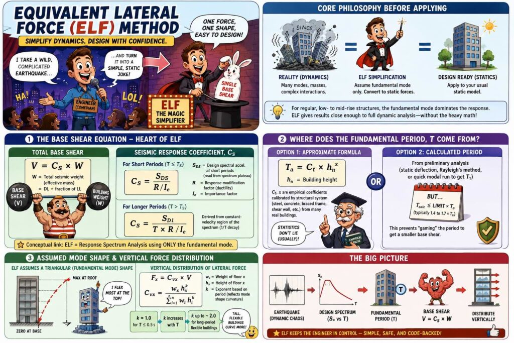
This is not an arbitrary simplification. It is built on the observation, confirmed by decades of dynamic analysis of real buildings, that for regular, reasonably low-rise structures the fundamental mode dominates the response so completely that the contribution of higher modes is small enough to be safely ignored or folded into conservative empirical factors.
For these structures, ELF gives results close enough to a full modal response spectrum analysis that the additional complexity of mode shapes, participation factors, and modal combination rules is simply not worth the effort.
The base shear equation — the heart of the method
The total seismic base shear is computed directly from a single formula:
V = Cs × W
Where W is the total seismic weight of the structure (essentially the same effective seismic mass used in modal analysis — full dead load plus an appropriate fraction of live load) and Cs is the seismic response coefficient, which plays exactly the same role that the spectral acceleration Sa played in response spectrum analysis, but evaluated using only the fundamental period rather than for every mode individually:
Cs = SDS / (R/Ie)
Where SDS is the design spectral acceleration parameter at short periods (read from the same underlying design spectrum used for response spectrum analysis, at the short-period plateau), R is the response modification factor (the same ductility-based reduction factor discussed under response spectrum analysis), and Ie is the importance factor.
For longer-period structures the coefficient transitions to a period-dependent form derived directly from the constant-velocity region of the design spectrum (the same 1/T decay described in the response spectrum design spectrum anatomy):
Cs = SD1 / (T × R/Ie)
This direct correspondence is the key conceptual link: ELF is not a fundamentally different physical model from response spectrum analysis — it is response spectrum analysis with only one mode (the fundamental mode) considered, and with that single mode’s spectral value read using a simplified, code-approximated fundamental period rather than one computed from a detailed eigenvalue analysis.
Why only the fundamental period, and where it comes from
Since ELF does not require modal analysis, the fundamental period itself must be estimated, not calculated from an eigenvalue problem. Codes provide two options:
The approximate period formula:
Ta = Ct × hₙˣ
Where hₙ is the building height and Ct, x are empirical coefficients calibrated by structural system (steel moment frame, concrete moment frame, braced frame, shear wall) from statistical regression against the measured periods of many real buildings — directly echoing the same empirical period-check formula introduced under modal analysis, used there as a sanity check on the computed eigenvalue results, but used here as the primary and only period estimate.
The properly calculated period from a preliminary structural analysis (such as a simple static deflection calculation, Rayleigh’s method, or even a quick modal analysis run purely to obtain T₁), which most codes permit as an alternative provided it does not exceed a specified upper bound multiple of the approximate period (commonly 1.4 to 1.7 times Ta, depending on the seismic design category) — a limit imposed specifically to prevent engineers from claiming an unrealistically long, overly flexible period in order to ride down the descending branch of the design spectrum and artificially reduce their design base shear.
The assumed mode shape — why ELF still has an implicit “mode”
Even though ELF performs no eigenvalue extraction, it still implicitly assumes a shape for how the building deforms — conventionally a linear, triangular distribution increasing from zero at the base to a maximum at the roof, which is a reasonable first-order approximation to the fundamental mode shape of a typical regular building (the same fundamental mode shape described under modal analysis: maximum displacement at the roof, zero at the base, no internal nodes). The vertical distribution formula reflects this assumed shape directly:
Fx = Cvx × V
Cvx = (wx hxᵏ) / Σ(wi hiᵏ)
Where wx and hx are the weight and height of floor x, and k is an exponent (1.0 for buildings with period ≤ 0.5 seconds, increasing toward 2.0 for longer-period, more flexible buildings, reflecting the fact that taller, more flexible structures have fundamental mode shapes that curve more strongly toward the top — a direct, simplified nod to the genuine mode-shape behavior that a full modal analysis would capture explicitly).
How the equivalent lateral force procedure is applied step by step
Step 1 — Determine the seismic design parameters for the site
Obtain the mapped spectral acceleration values for the site (SS at short period and S1 at one-second period) from the relevant national or regional seismic hazard maps, then apply site coefficients (Fa and Fv, based on the site soil classification, exactly as described under the response spectrum design spectrum) to obtain the site-adjusted design spectral accelerations SDS and SD1.
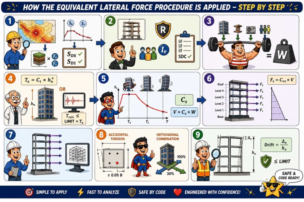
Step 2 — Determine the structural design parameters
Identify the appropriate response modification factor R based on the structural system and detailing (the identical R-factor discussed at length under response spectrum analysis, governing the trade-off between elastic design force and assumed ductile capacity), the importance factor Ie based on the building’s risk category, and the seismic design category, which governs which analysis procedures are even permitted for this particular structure.
Step 3 — Compute the total seismic weight W
Sum the effective seismic weight of the entire structure — dead load of all structural and non-structural components, plus the appropriate fraction of live load and storage load specified by the applicable code, exactly as described for the mass model under modal analysis, since this is fundamentally the same seismic mass, just expressed as a weight (mass times gravity) rather than as a mass matrix.
Step 4 — Estimate the fundamental period
Using either the approximate empirical formula Ta or a properly calculated period subject to the code’s upper-bound limit, as described above.
Step 5 — Compute the seismic response coefficient Cs and the total base shear V
Apply the governing formula for Cs based on where the estimated period falls relative to the characteristic periods of the design spectrum (the short-period plateau, the constant-velocity descending branch, or — for very long-period or very short-period structures — the special minimum and maximum limits that codes impose to prevent unrealistically low or unbounded design forces). Multiply by W to obtain the total design base shear V.
Step 6 — Distribute the base shear vertically to each floor level
Apply the Cvx distribution formula to allocate the total base shear V into individual floor-level forces Fx, concentrated at each floor’s center of mass, following the assumed (triangular or near-triangular) mode shape described above.
Step 7 — Apply the floor forces to a static structural model
With the seismic forces now expressed as ordinary static point loads at each floor level, the entire remainder of the analysis is conventional linear static structural analysis — exactly the same FEM or hand-calculation procedure used for gravity or wind loads, with no further dynamic content whatsoever. Member forces, story shears, overturning moments, and displacements are all found through standard static equilibrium and stiffness methods.
Step 8 — Check accidental torsion and orthogonal load combinations
Codes typically require the lateral force at each floor to be applied with a small assumed eccentricity (accidental torsion, commonly 5% of the building dimension perpendicular to the direction of loading) to account for uncertainties in mass and stiffness distribution not explicitly captured by the simplified analysis, and require combining the primary direction loading with a percentage of the orthogonal direction loading — the same directional combination requirement described under response spectrum analysis, applied here to the static force pattern instead of to dynamically combined modal responses.
Step 9 — Check drift limits
Story drifts computed from the static analysis under the ELF forces (often after first dividing by the deflection amplification factor Cd, a companion factor to R that governs how much the elastic ELF-computed displacement must be amplified to estimate the actual expected inelastic displacement) are checked against code drift limits, exactly as described under response spectrum analysis, using the identical drift limit values and the identical underlying philosophy.
Key characteristics and limitations to understand
It assumes the fundamental mode dominates completely
ELF contains no mechanism whatsoever for capturing higher mode contributions. For genuinely regular, low-rise buildings, where the fundamental mode does capture the overwhelming majority of the dynamic response (the same mass participation principle established under modal analysis, but here assumed rather than verified), this is an acceptable approximation.
For taller or more irregular buildings, where higher modes contribute meaningfully, ELF can significantly misrepresent both the magnitude and the distribution of the true dynamic forces — which is precisely why codes restrict its use to structures below specified height and regularity thresholds, escalating to mandatory modal response spectrum analysis beyond those thresholds.
It cannot represent torsional irregularity or coupled modes properly
Because ELF applies forces independently at each floor’s center of mass based only on a simplified vertical mode shape, it has no inherent mechanism to capture coupled torsional-translational behavior (the same phenomenon flagged as identifiable directly from modal analysis mode shapes).
The accidental torsion provision is a blunt, empirical patch for this limitation, not a genuine dynamic representation of torsional response — which is exactly why codes require escalation to dynamic analysis once torsional irregularity exceeds specified thresholds.
It is, like response spectrum analysis, fundamentally a linear elastic method relying on the R-factor
Exactly as described for response spectrum analysis, ELF computes an elastic-equivalent force level and then relies entirely on the empirical response modification factor R to account for the structure’s assumed ductile capacity to survive the much larger true elastic demand through controlled yielding.
ELF does not add any additional nonlinear sophistication beyond what response spectrum analysis already provides through this same R-factor mechanism — it simply estimates the elastic demand even more crudely, using a single assumed mode rather than a full set of computed modes.
It uses an estimated, not computed, fundamental period
Because no eigenvalue analysis is performed, the period used to enter the design spectrum is an empirical estimate rather than a calculated property of the actual structural model.
This is a deliberate, conservative design choice by code committees — the empirical period formulas are generally calibrated to produce shorter (stiffer) period estimates than a detailed structural model would actually compute, which pushes the design point further up the steeply rising short-period portion of the spectrum and produces a larger, more conservative base shear than a more accurate period estimate would give. This conservatism is precisely the safety margin that allows codes to permit ELF without requiring the more rigorous modal eigenvalue extraction.
Application cases in structural engineering
Regular, low-rise to mid-rise buildings — the overwhelming majority of applications
The single most common application worldwide: standard residential buildings, small to medium commercial structures, schools, and warehouses with regular plan and vertical configurations, typically up to a height threshold that varies by code and seismic design category (commonly around 50 to 75 m or a specified number of stories, though the exact limit depends on seismic design category, structural system, and regularity classification).
For the vast number of low-rise and many mid-rise buildings constructed every year, ELF is not merely permitted but is by far the most frequently used seismic design method in practice, precisely because most ordinary buildings fall comfortably within the regularity and height limits where the fundamental-mode-only assumption is well justified.
Preliminary design and conceptual sizing of all building types, including those that will ultimately require dynamic analysis
Even for taller or more complex buildings that will ultimately be designed using modal response spectrum analysis or nonlinear time history analysis, ELF is almost universally used first, during conceptual and preliminary design, to obtain quick, hand-calculable estimates of base shear and approximate member forces before any detailed dynamic model exists.
This mirrors exactly the role described for response spectrum analysis within performance-based design frameworks — ELF sits one level even further upstream, as the very first dynamic-equivalent estimate an engineer reaches for before investing in any eigenvalue extraction at all.
The mandatory minimum base shear check on dynamic analysis results
As established under both response spectrum analysis and time history analysis, virtually every code requires that the base shear obtained from any more sophisticated dynamic procedure be compared against a minimum value derived from the ELF base shear formula (commonly requiring the dynamic base shear to be no less than 85% of the ELF value, scaling up the dynamic results if necessary).
This means ELF is not simply an alternative to dynamic analysis for simple buildings — it is embedded as a mandatory floor-level check within every single modal response spectrum and, in many jurisdictions, time history analysis performed on every building of every height and complexity, making it arguably the most universally applied seismic calculation in the entire profession even though it is rarely the final governing analysis for complex structures.
Wind and seismic comparison studies for low and mid-rise structures
Because ELF produces a simple static force distribution directly comparable in form to a static wind load pattern, it is the natural tool engineers reach for when performing quick comparative studies of whether wind or seismic loading governs the lateral design of a particular structure, before committing to the more detailed analysis (whether wind tunnel testing and gust factor methods, or modal response spectrum analysis) that the governing load case will ultimately require.
Non-building structures and simple industrial structures
Pipe racks, equipment platforms, storage tanks, and other non-building structures that are reasonably regular and do not fall into specially restricted categories are frequently designed using ELF-based procedures adapted from the building code provisions, exactly because these structures typically behave with strong fundamental-mode dominance similar to regular low-rise buildings, and the cost and complexity of full modal analysis is rarely justified for these simpler industrial structures.
Retrofit screening and rapid seismic vulnerability assessment
For large portfolios of existing buildings (school district seismic safety programs, municipal building inventories, insurance company portfolio risk assessments), ELF-based procedures provide a rapid, standardized, and inexpensive method for screening large numbers of structures to identify which ones warrant more detailed investigation — directly analogous to the role described for response spectrum analysis in preliminary seismic evaluation of existing buildings, but applied here at an even earlier and coarser screening stage, often before any detailed structural model of the existing building has even been built.
How the equivalent lateral force procedure fits into modern earthquake design practice
It is the entry point and the floor of the entire code hierarchy
Returning to the four-tier hierarchy established under response spectrum analysis and refined under time history analysis — equivalent lateral force, then modal response spectrum analysis as the default workhorse, then linear time history as an occasional refinement, then nonlinear time history for performance-based verification of critical structures — ELF sits at both the bottom and, in a different sense, underneath the entire structure.
It is the bottom tier in terms of sophistication and the threshold below which more rigorous methods are not required, but it is also literally underneath every tier above it, because its minimum base shear value constrains and validates the results of every more sophisticated method performed on top of it.
Why it has survived essentially unchanged in principle for over half a century
The core logic of ELF — total base shear from a simplified coefficient times weight, distributed vertically by an assumed shape — has remained conceptually stable since its earliest codified forms in the mid-20th century, even as the underlying hazard maps, spectral shapes, and R-factor values have been repeatedly refined and updated based on improved seismological understanding and observed earthquake performance.
This longevity exists for the same fundamental reasons response spectrum analysis remains dominant over nonlinear time history, taken one step further: ELF requires no software, no eigenvalue solver, and can be performed by hand or on a simple spreadsheet by any licensed engineer anywhere in the world, regardless of access to specialized dynamic analysis software — a practical accessibility consideration that remains critically important for the enormous volume of ordinary, regular buildings constructed in every country, including those with less access to sophisticated engineering software and computational resources.
Its relationship to the R-factor and ductility framework — identical to response spectrum analysis, but even more dependent on it
Exactly as described for response spectrum analysis, ELF computes an elastic-equivalent force that is deliberately reduced by the response modification factor R to obtain a design force far below the true elastic earthquake demand, relying entirely on assumed ductile detailing to survive the actual demand through controlled yielding.
Because ELF’s estimate of the elastic demand itself is already a cruder approximation than response spectrum analysis (single assumed mode versus genuine multi-modal combination, estimated period versus calculated eigenvalue), ELF leans even more heavily on the conservatism built into the R-factor framework and the empirical period formulas to compensate for its own simplifications — meaning the entire safety margin of ELF design depends on the cumulative conservatism baked into multiple linked empirical factors (period formula, R-factor, importance factor, minimum base shear limits) working together, rather than on any single rigorous dynamic calculation.
Its diminishing but still foundational role as building height and complexity increase
As established progressively through response spectrum analysis and time history analysis, the profession’s reliance on ELF diminishes steadily as structures become taller, more irregular, or more critical — exactly mirroring the escalating tiers of the code hierarchy.
Yet even at the very top of that hierarchy, in the nonlinear time history analysis of a critical essential facility or a supertall tower with novel damping systems, the ELF base shear calculation is still typically the very first number computed, used as an immediate sanity check, a preliminary sizing tool, and — in most jurisdictions — a mandatory minimum floor that the final, far more sophisticated analysis results must still respect.
In this sense ELF is not merely the simplest method in the hierarchy but the universal common denominator underlying every seismic design performed anywhere in the profession, regardless of how far up the sophistication ladder the final design analysis ultimately climbs.
Comparison with related dynamic analysis methods
| Aspect | Equivalent lateral force | Response spectrum analysis | Linear time history | Nonlinear time history |
| Modes considered | Fundamental mode only (assumed shape, not computed) | Multiple modes explicitly combined | All modes via modal superposition or direct integration | All modes, with changing stiffness |
| Period source | Empirical formula or simplified estimate (capped) | Computed eigenvalue analysis | Computed eigenvalue analysis | Computed eigenvalue analysis (initial elastic state) |
| Captures higher modes | No | Yes | Yes | Yes |
| Captures torsional/coupled behavior | No — only via blunt accidental torsion provision | Yes — directly from mode shapes | Yes | Yes |
| Captures time sequence | No | No — peaks only | Yes — complete history | Yes — complete history |
| Captures nonlinearity | No (R factor applied empirically) | No (R factor applied empirically) | No | Yes — explicitly modeled |
| Required input | Code seismic coefficient and weight only | Single design spectrum | Multiple ground motion records | Multiple ground motion records plus nonlinear element models |
| Computational cost | Negligible — hand calculation feasible | Low to moderate | Moderate | High to very high |
| Engineering judgment required | Minimal | Moderate (spectrum selection) | Significant (record selection/scaling) | Extensive (records, hysteretic models, convergence) |
| Code requirement trigger | Regular, low-rise to mid-rise buildings | Tall, irregular buildings; most bridges | Critical structures, site-response studies | Performance-based design, essential facilities, base isolation |
| Frequency of real-world use | Extremely common for ordinary buildings; universal as preliminary/minimum check | The most common method for final design of complex structures | Occasional, specialist studies | Rare, reserved for critical/high-consequence structures |
Summary in one sentence
The equivalent lateral force procedure is a simplified method of earthquake analysis that is commonly used for low rise buildings. It is applied by estimating the fundamental period from an empirical code formula, reading the corresponding seismic response coefficient from the same design spectrum used in response spectrum analysis but considering only this single assumed fundamental mode.
The lateral forces are estimated from the total base shear that is computed multiplying this coefficient by the building’s effective seismic weight, and it is distributed vertically among floor levels using a simplified triangular approximation to the fundamental mode shape. The resulting forces are applied as ordinary static loads to a conventional structural model.
The method serves as not merely the simplest and most accessible seismic design method available, requiring no eigenvalue extraction, no ground motion selection, and no specialized dynamic analysis software. But it also forms the universal foundation embedded as a mandatory minimum check beneath every more sophisticated method in the seismic design hierarchy, remaining today.
It is the primary and sufficient method of demonstrating seismic code compliance, for the vast majority of regular, low-rise to mid-rise structures built throughout the world, while serving simultaneously as the indispensable first preliminary estimate and the ever-present conservative floor constraining the results of modal response spectrum analysis, linear time history analysis, and even nonlinear time history analysis performed on the most complex and critical structures in the profession.