
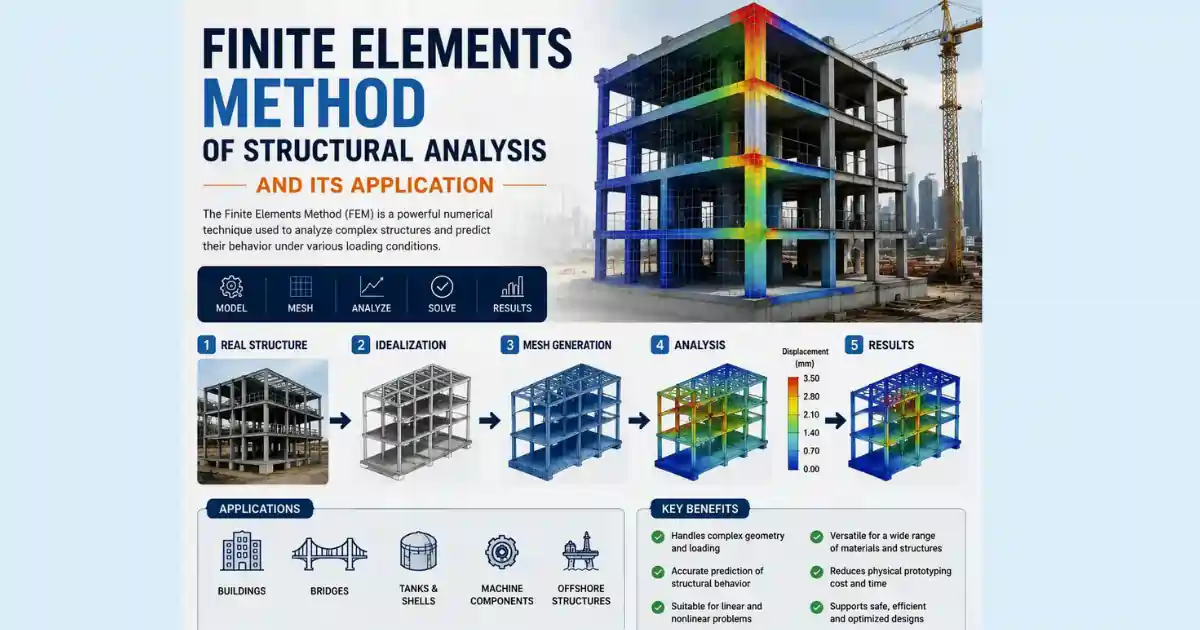
The finite element method of analysis is the most general and powerful structural analysis method ever developed. Most leading engineering softwares use the method because it made modern engineering possible by allowing analysis of structures of arbitrary shape, material, loading, and boundary conditions that no classical method could ever handle.
The finite element method works by asking one fundamental question about any complex structure: “can we divide it into small simple pieces, solve each piece approximately, connect them all together, and get a good approximation of the whole structure’s behavior?”
What is the Core philosophy for Finite Element Method
The Core idea
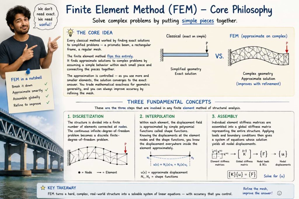
Every classical method worked by finding exact solutions to simplified problems — a prismatic beam, a rectangular frame, a regular plate. The finite element method flips this entirely. It finds approximate solutions to complex problems by assuming a simple behavior within each small piece and connecting the pieces together.
The approximation is controlled — as you use more and smaller elements, the solution converges to the exact answer. You trade mathematical exactness for geometric generality, and you can always improve accuracy by refining the mesh.
Finite element method is usually offered in graduate courses and the softwares such as MATLAB and ABACUS are used in solving problems.
Matlab is a code that is used in solving FEM problems that is helpful since when the number of elements becomes larger the only way of solving them is by computing. ABACUS is a FEM software that is also used professionally to design structures and mechanical products.
Both MATLAB and ABACUS use as their foundation FEM principles, the only difference is MATLAB is applied as coding but ABACUS has also a visual UI option.
Three fundamental concepts in FEM
These are the three steps that are involved in any finite element method of structural analysis.
1.Discretization — the structure is divided into a finite number of elements connected at nodes. The continuous infinite-degree-of-freedom problem becomes a discrete finite-degree-of-freedom problem.
2.Interpolation — within each element, the displacement field is approximated by simple polynomial functions called shape functions. Knowing the displacements at the element nodes and the shape functions, you know the displacement everywhere inside the element approximately.
3.Assembly — individual element stiffness matrices are assembled into a global stiffness matrix representing the entire structure. Applying loads and boundary conditions then gives a system of equations whose solution yields all nodal displacements.
Mathematical foundation
The principle of virtual work
The finite element method is grounded in the principle of virtual work — for a structure in equilibrium, the work done by external forces through any virtual displacement equals the internal strain energy stored. This variational principle is more general than direct equilibrium and naturally handles complex 3D stress states.
Before jumping into 3D elasticity, it’s clearest to see the principle of virtual work on a simple 1D bar (axial member), since all the same ideas carry over directly.
1D FEM Example Setup
Consider a bar of length L, cross-sectional area A, Young’s modulus E, fixed at one end, with an axial displacement field u(x). The strain is:
ε(x) = du/dx
and the stress is:
σ(x) = E ε(x)
Virtual work statement
The principle says: for the bar in equilibrium, if we impose any virtual (imaginary, kinematically admissible) displacement δu(x), the external virtual work equals the internal virtual work (strain energy):
∫ σ δε A dx = ∫ f δu dx + P δu(L)
where f is a distributed axial load and P is a point load at the tip. The left side is internal virtual work; the right side is external virtual work.
Discretizing with shape functions
In FEM, we approximate the displacement inside an element using nodal values {u} and shape functions [N]:
u(x) = [N]{u}
Differentiating to get strain, we define the strain-displacement matrix [B] = d[N]/dx, so:
ε(x) = [B]{u}
Since [B] is constant for a 2-node linear bar element, this is simple. Substituting σ = E ε = E[B]{u} into the virtual work statement, and letting the virtual displacement also be discretized as δu(x) = [N]{δu}, gives:
{δu}ᵀ ∫ [B]ᵀ E [B] A dx {u} = {δu}ᵀ {f}
Since {δu} is arbitrary, we can cancel it from both sides, leaving the element equilibrium equation:
∫ [B]ᵀ [D] [B] A dx {u} = {f}
where [D] = E (just a scalar in 1D — the “constitutive matrix” reduces to Young’s modulus). This is exactly the 1D version of the general element stiffness equation:
[k]{u} = {f}, with [k] = ∫ [B]ᵀ [D] [B] A dx
Why this matters for going to 3D
Notice the structure of the final equation:
∫ [B]ᵀ [D] [B] dV {u} = {f}
is identical in form whether you’re in 1D, 2D, or 3D. What changes going to 3D is:
- {u} becomes a vector of nodal displacements in x, y, z (not just axial)
- ε and σ become full strain/stress tensors written as vectors (6 components each, using engineering notation)
- [B] becomes a matrix that relates nodal displacements to all strain components (not just du/dx)
- [D] becomes the full elasticity (constitutive) matrix relating stress to strain (incorporating E, ν, shear modulus, etc.), not just a scalar E
So the 1D bar already contains the complete logical skeleton of the FEM virtual work formulation — the jump to 3D is really just “more components per node, and a bigger [B] and [D].”
For a single element in 3D: ∫∫∫ [B]ᵀ[D][B] dV {u} = {f}
Where:
- [B] = strain-displacement matrix (derivatives of shape functions)
- [D] = material constitutive matrix (relates stress to strain)
- {u} = nodal displacement vector
- {f} = nodal force vector
The integral [k] = ∫∫∫ [B]ᵀ[D][B] dV is the element stiffness matrix — the fundamental building block of the entire method.
Shape functions
Shape functions Nᵢ(x,y,z) interpolate the displacement field within an element from the nodal values. For a two-node bar element with nodes at x = 0 and x = L:
N₁ = 1 − x/L (equals 1 at node 1, 0 at node 2) N₂ = x/L (equals 0 at node 1, 1 at node 2)
Displacement at any point: u(x) = N₁u₁ + N₂u₂
For higher-order elements, shape functions are quadratic, cubic, or higher polynomials, giving better accuracy with fewer elements.
Strain and stress recovery
Strains are derivatives of displacements: {ε} = [B]{u} where [B] = d[N]/dx (or appropriate derivatives in 2D/3D)
Stresses follow from the constitutive law: {σ} = [D]{ε} = [D][B]{u}
This is how FEM recovers stresses from the primary unknown displacements.
Element types — the building blocks
1D elements
Bar element — carries axial force only, two nodes, one DOF per node (axial displacement). Used for trusses and cables.
Beam element — carries bending moment and shear, two nodes, two DOFs per node (transverse displacement and rotation). The Euler-Bernoulli beam element is the direct matrix version of the slope-deflection method. The Timoshenko beam element adds shear deformation for deep beams.
Frame element — combines bar and beam, three DOFs per node in 2D (axial, transverse, rotation), six DOFs per node in 3D. Used for building and bridge frames.
2D elements
Plane stress element — for thin plates loaded in their own plane (membrane action). Triangular (CST — constant strain triangle, LST — linear strain triangle) or quadrilateral (Q4 bilinear, Q8 serendipity). Two DOFs per node (u, v displacements).
Plane strain element — for long structures where out-of-plane strain is zero (dams, tunnels, retaining walls). Same element shapes as plane stress, different [D] matrix.
Plate bending element — for flat plates carrying transverse loads by bending. Three DOFs per node (transverse displacement w, two rotations). Kirchhoff plate for thin plates, Mindlin plate for thick plates including shear deformation.
Shell element — combines membrane and bending, handles curved surfaces. Five or six DOFs per node. Used for domes, tanks, curved bridges, aircraft fuselages.
3D elements
Solid elements — tetrahedral (4 or 10 nodes) or hexahedral brick (8 or 20 nodes). Three DOFs per node (u, v, w). Used for massive structures, soil volumes, machine parts where full 3D stress state is needed.
Special elements
Spring element — one DOF, represents foundation stiffness or connection flexibility. Gap element — zero stiffness in tension, full stiffness in compression. Used for contact problems. Interface element — models thin layers between materials, bond-slip in reinforced concrete. Infinite element — extends mesh to infinity for soil and unbounded domains.
The Basic and widely applied form of FEM, Linear static analysis
Linear static analysis is the simplest and most widely used form of finite element analysis. It assumes that materials remain linearly elastic, deformations are small enough that the structure’s geometry does not significantly change, and loads are applied slowly so that dynamic effects such as inertia and damping can be neglected.
Under these assumptions, structural response is directly proportional to the applied load, making the analysis both efficient and reliable for many engineering applications.
The basic case involves one load vector and one solution. Because the stiffness matrix remains constant throughout the analysis, the system of equations is solved only once to obtain nodal displacements, from which strains, stresses, and support reactions are determined.
Linear static analysis is suitable for structures that remain within the elastic range and experience relatively small displacements under static loading. Most of building structural design falls in this category.
How FEM is applied step by step
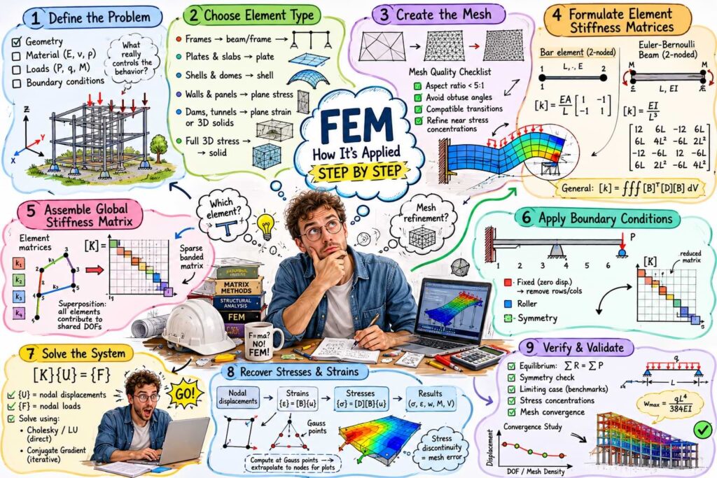
Step 1 — Define the problem
Establish the geometry, material properties, loading, and boundary conditions. Decide which structural behavior governs — is it primarily bending (use beam or plate elements), membrane action (use plane stress), full 3D stress (use solid elements), or a combination?
Simplify where possible. A symmetric structure under symmetric loading needs only half the model — apply symmetry boundary conditions at the axis of symmetry. An antisymmetric load on a symmetric structure needs only half the model with antisymmetric boundary conditions.
Step 2 — Choose element type
Match the element type to the physics:
- Framed structures → beam/frame elements
- Thin flat plates and slabs → plate bending elements
- Curved shells, domes, tanks → shell elements
- Deep beams, walls, shear panels → plane stress elements
- Dams, embankments, tunnels → plane strain or 3D solid elements
- Full 3D stress states → solid elements
Using a higher-dimensional element than necessary wastes computation. Using a lower-dimensional element than the physics requires gives wrong answers. Getting this choice right is one of the most important engineering judgments in FEM.
Step 3 — Create the mesh
Divide the geometry into elements. Mesh density controls accuracy — finer mesh near stress concentrations, boundaries, load application points, and regions of rapid stress variation. Coarser mesh is acceptable where behavior is smooth and gradual.
Mesh quality matters as much as mesh density:
- Avoid highly distorted elements — aspect ratios greater than 5:1 reduce accuracy
- Avoid very obtuse angles in triangular elements
- Ensure compatible meshes — nodes of one element must not sit on the edge of an adjacent element without being connected
- Transition gradually from fine to coarse mesh regions
Step 4 — Formulate element stiffness matrices
For each element, compute the stiffness matrix [k] = ∫∫∫ [B]ᵀ[D][B] dV. For simple elements like bars and Euler-Bernoulli beams this integral has a closed-form result. For 2D and 3D elements it is evaluated numerically using Gauss quadrature — a method of approximating integrals by evaluating the integrand at specific points called Gauss points and weighting the results.
For a two-node bar element of length L, area A, modulus E: [k] = (EA/L) × [1 −1; −1 1]
For a two-node Euler-Bernoulli beam element of length L, EI: [k] = (EI/L³) × [12, 6L, −12, 6L; 6L, 4L², −6L, 2L²; −12, −6L, 12, −6L; 6L, 2L², −6L, 4L²]
This 4×4 matrix is the direct matrix equivalent of the slope-deflection equations — the slope-deflection stiffness coefficients 4EI/L, 2EI/L, 6EI/L² and 12EI/L³ appear explicitly in its entries.
Step 5 — Assemble the global stiffness matrix
Each element stiffness matrix contributes to the global stiffness matrix [K] by adding its entries to the appropriate rows and columns corresponding to the global DOF numbers of its nodes.
This assembly process — often called the direct stiffness method — works by the principle of superposition: the global stiffness matrix represents the combined resistance of all elements to nodal displacements. Elements sharing a node both contribute to the rows and columns of that node.
The result is a large sparse symmetric banded matrix. For a beam with n nodes, [K] is 2n × 2n with non-zero entries only within a narrow band around the diagonal.
Step 6 — Apply boundary conditions
Prescribed displacement boundary conditions (fixed supports, roller supports, symmetry conditions) are applied by modifying the global stiffness matrix and load vector. The most common method is to delete the rows and columns corresponding to prescribed zero displacements, reducing the system size.
For non-zero prescribed displacements (support settlements), transfer the known displacement terms to the right hand side of the equation.
Natural boundary conditions — applied forces and moments — are simply added directly to the load vector at the corresponding DOFs.
Step 7 — Solve the system of equations
[K]{U} = {F}
Where {U} is the global displacement vector and {F} is the global load vector. For linear static analysis this is solved once using direct methods like Cholesky factorization or LU decomposition, exploiting the banded sparse structure for efficiency.
For large models with millions of DOFs, iterative solvers like conjugate gradient methods are used instead, since they do not require storing the full matrix.
Step 8 — Recover stresses and strains
From nodal displacements, compute element strains using {ε} = [B]{u} and stresses using {σ} = [D][B]{u}. Stresses are typically computed at Gauss points first — where they are most accurate — then extrapolated to nodes for visualization.
Nodal stresses from adjacent elements will generally not be identical — the discontinuity is a measure of mesh error. Averaging nodal stresses from surrounding elements gives smoother results. Large discontinuities indicate the mesh needs refinement in that region.
Step 9 — Verify and validate
Check equilibrium — sum of support reactions should equal applied loads. Check symmetry — symmetric loads on symmetric structures should give symmetric results. Check limiting cases — a simply supported beam under uniform load should give wL⁴/384EI at midspan. Check stress concentrations — stresses near sharp corners should be high but finite — truly infinite stresses indicate a mesh singularity. Perform mesh convergence study — refine the mesh and check that results stabilize.
Analysis types beyond linear static
In these types of analysis the assumptions for linear statics do not hold. Most structural design falls under linear statics design. However, when the actual conditions do not warrant the assumptions the specific FEM design is applied.
Modal analysis — natural frequencies and mode shapes
Solve the eigenvalue problem: ([K] − ω²[M]){φ} = 0
Where [M] is the mass matrix assembled similarly to [K], ω are natural frequencies, and {φ} are mode shapes. Essential for earthquake engineering, vibration design, and dynamic response analysis.
Response spectrum analysis
Combines modal analysis with a design spectrum to find maximum seismic response. Each mode is analyzed separately and results are combined using SRSS or CQC combination rules. Standard method for seismic design of buildings and bridges.
Time history analysis
Integrate the equation of motion [M]{Ü} + [C]{U̇} + [K]{U} = {F(t)} step by step through time. Used for detailed seismic analysis, blast loading, impact, and any time-varying loading where response spectrum is insufficient.
Buckling analysis
Solve the eigenvalue problem: ([K] + λ[Kᵍ]){φ} = 0
Where [Kᵍ] is the geometric stiffness matrix accounting for the destabilizing effect of compressive forces. The lowest eigenvalue λ gives the buckling load multiplier. Used for slender columns, thin plates, and shells under compression.
Nonlinear static analysis
For material nonlinearity (plasticity, cracking, crushing) or geometric nonlinearity (large deflections, P-delta effects), the stiffness matrix changes as loads increase. The solution proceeds incrementally — apply load in steps, update [K] at each step, iterate to convergence within each step using Newton-Raphson or arc-length methods.
Pushover analysis
Nonlinear static analysis under monotonically increasing lateral loads. Used in earthquake engineering to assess structural ductility, identify failure mechanisms, and determine the collapse load of building frames. The load-displacement curve (pushover curve) shows how the structure transitions from elastic to inelastic behavior.
Nonlinear dynamic analysis
The most computationally demanding analysis type — combines time-stepping integration with nonlinear material and geometric behavior updated at every time step. Used for detailed seismic performance assessment, progressive collapse analysis, and blast response.
Heat transfer analysis
The same mathematical framework applies — replace the stiffness matrix with a conductivity matrix, replace displacements with temperatures, replace forces with heat fluxes. Transient heat transfer adds a capacitance matrix analogous to the mass matrix. Used for fire analysis, thermal bridging, and coupled thermo-mechanical problems.
Fluid-structure interaction
Combines structural FEM with computational fluid dynamics — the fluid pressure loads the structure, the structure deformation changes the fluid domain, and the two solutions are coupled iteratively. Used for bridge aeroelasticity, offshore platforms, dam-reservoir interaction, and heart valve analysis.
Where FEM works best
The application of FEM excels where analytical methods become cumbersome or difficult. FEM is adopted to solve those more complex problems in diverse civil engineering fields.
Complex geometry
Curved bridges, shell roofs, folded plates, irregular plan shapes, openings in walls and slabs — any geometry that classical methods cannot handle is natural territory for FEM. The mesh conforms to any shape.
Stress concentration analysis
Near holes, notches, re-entrant corners, load introduction points, and connection details, stresses vary rapidly. A refined FEM mesh resolves these gradients accurately. Classical methods give only average member forces and cannot capture local peak stresses.
Plate and shell structures
Flat slabs, curved roof shells, pressure vessels, storage tanks, ship hulls, aircraft fuselages — all are governed by 2D or curved surface behavior that requires plate or shell elements. No classical hand method can analyze these rigorously.
Soil-structure interaction
The soil beneath a foundation is a continuous deformable medium. Modeling it with solid elements or spring elements coupled to structural elements captures the redistribution of pressure under a raft foundation, the settlement profile under an embankment, or the lateral earth pressure on a retaining wall.
Seismic analysis
The combination of modal analysis, response spectrum, and nonlinear time history analysis — all implemented in FEM — forms the complete toolkit for modern seismic design. No other method provides this range of analysis capability.
Progressive collapse analysis
When a key structural element is suddenly removed, the remaining structure must redistribute forces through alternative load paths. Nonlinear dynamic FEM analysis tracks this redistribution and identifies whether collapse is arrested or propagates. Essential for design of critical infrastructure.
Connection and detail design
Beam-column connections, anchor plates, gusset plates, and other connection details develop complex 3D stress states that beam theory cannot capture. Solid element models of connections give the full stress distribution for fatigue assessment and ultimate capacity evaluation.
Composite and layered structures
Reinforced concrete combines steel and concrete with different material properties. Laminated composites have different properties in different directions and through the thickness. FEM handles multi-material and anisotropic problems naturally through the [D] matrix.
Nonlinear material behavior
Concrete cracking and crushing, steel yielding, soil plasticity, rubber hyperelasticity — all require nonlinear constitutive models that enter through the [D] matrix update at each load step. No classical method handles material nonlinearity.
Temperature effects and thermal loads
Thermal expansion, temperature gradients through cross-sections, fire loading — all are handled by coupling thermal and structural analyses. The thermal analysis gives temperature distributions; the structural analysis converts them to thermal strains and stresses.
Where it struggles or requires care
Mesh dependency in nonlinear problems
In strain softening materials — concrete after cracking, soil after peak strength — the numerical solution can become mesh dependent. Finer meshes give different results rather than converging. Special regularization techniques like crack band models or non-local formulations are needed.
Locking phenomena
Certain element formulations suffer from artificial stiffness called locking. Shear locking occurs in thin beam and plate elements when low-order polynomials cannot represent pure bending without spurious shear strains. Volumetric locking occurs in nearly incompressible materials. These pathological behaviors require special element formulations — reduced integration, mixed formulations, or enhanced strain elements — to overcome.
Stress singularities
At sharp re-entrant corners and crack tips, the theoretical stress is infinite. FEM produces very high but finite stresses that increase indefinitely as the mesh is refined. This is physically correct for cracks — fracture mechanics uses the stress intensity factor extracted from the singular field — but for general re-entrant corners it signals a modeling error that should be resolved by adding a fillet radius.
User expertise required
Unlike classical methods that give clear warnings when misapplied, FEM will produce plausible-looking but wrong results from incorrect element choice, poor mesh quality, wrong boundary conditions, or inappropriate material models. Garbage in, garbage out applies powerfully. Verification and validation are not optional.
Computational cost for very large nonlinear dynamic models
A detailed nonlinear time history analysis of a full building under a long earthquake record can take hours or days even on modern computers. Simplifications — reduced models, substructuring, surrogate models — are often necessary for practical design applications.
Comparison with all other methods
| Aspect | FEM | Finite difference | Classical methods |
| Geometry | Arbitrary | Regular mesh | Simple members |
| Element types | Bars, beams, plates, shells, solids | Uniform mesh points | Member types only |
| Material nonlinearity | Full support | Possible but complex | Not supported |
| Geometric nonlinearity | Full support | Possible | Very limited |
| Dynamic analysis | Full support | Possible | Very limited |
| Stress concentrations | Excellent with mesh refinement | Poor — needs very fine mesh | Cannot capture |
| Mesh refinement | Local refinement possible | Uniform only | Not applicable |
| 3D problems | Natural | Impractical | Not possible |
| Programming complexity | High — but commercial software available | Low | Not programmed |
| Physical insight | Low — results not intuitive | Low | High |
| Verification difficulty | High — many ways to get wrong answers | Moderate | Low |
| Best application | Any complex real-world structure | Regular 2D problems, teaching | Understanding, preliminary design, checking |
Summary in one sentence
The finite element method is at its most powerful for any structure where geometry, loading, material behavior, or boundary conditions are too complex for classical methods — which in practice means virtually every real engineering structure — and its combination of generality, accuracy, and the ability to handle static, dynamic, linear, and nonlinear behavior in 1D, 2D, and 3D makes it the universal language of modern structural analysis.